![]()
The Random Forests algorithm (RF) implemented in R via the randomForest package, is quite possibly the most data driven algorithm in existense today. Its high popularity stems from its excellent overall performance in prediction. However, due to its statistical complexity it is in general difficult to understand variable or feature contribution to the prediction. In addition, due to the variable random selection that occurs internally on each fully grown tree, RFs are not truly capturing higher order interaction effects. The exception to this are 2 way interactions where the effect is indeed captured.
Nonetheless, there have been efforts to alleviate such difficulties, and one such noble effort has been implemented and described in the R package forestFloor.
This package currently uses the results of forestFloor, hence it is advised that the user goes through forestFloor first, in order to better understand its theory and usage. Equipped with that knowledge, the user can then more easily transition to vis2rfi.
vis2rfi extracts Random Forest feature contributions that are computed in forestFloor, and combines them in order to do specifically one thing :
- Create 3 dimensional objects and/or surfaces that aim to describe the interaction effect of two variables on the predicted outcome.
The package’s name is shorthand for Visualising 2 Way Random Forest Interactions.
forestFloor implements a function for the same purpose, namely forestFloor::show3d, which is using rgl to create the visualisation. Here the approach taken is different (explained below), while the plotting tool is plotly.
Premise
- The package emphasizes the premise that when looking at a 3d visual it is often more effective to view the 2 way interaction effect as a 3d object instead of the usual 3d surface.
Premonitions With 3d Surface Depictions
When constructing 3d visualizations with thousands of data points, the following issues might arise:
Trends or curvatures in the produced surface are hard to be discerned. Viewing slices of the 3d surface can help in better extracting any potential interaction effect.
The sheer data volume might either crash the session or render it in a non-responsive state.
The 3d surface produced in an interactive display becomes more difficult to manipulate e.g. to turn the surface to a different viewing angle or to zoom in/‘out of’ it.
The computational time required to construct and to manipulate a 3d surface becomes longer. In applications one would like to manipulate the surface relatively fast so as to quicker extract any interaction effect that is present.
To tackle these issues subsampling is used together with smoothing in order to construct an approximation to the “all data” interaction effect, quicker and without significant loss of information.
Subsampling Approaches
The following subsampling approaches are implemented:
- Random Subsampling :
Take a random sample of the cases in the observed data set and use that to construct the 3d interaction effect object and/or surface of a pair of random forest important variables.
- Random Subsampling And GAM Smoothing :
Similarly as above but in addition fit a feature contribution smoother to the subsample, then resample from this smoother and construct the 3d surface on a more regularly sampled grid in the XY plane than the one observed in the original subsample. This way a smoother 3d interaction effect surface can be constructed.
- Random Subsampling With Maximum Dissimilarity Sampling :
Split a hypothetical random sample of cases in two parts: The base part and the pool part.
Fill the base part with a portion of the hypothetical random sample of observed cases (say 67%) and let the rest (say 33%) pool part be filled by other observed cases that are maximally separated (i.e. via the Euclidean distance) from the cases in the base part.
In this way, a more diverse range of feature contribution values can be obtained and hence a more accurate 3d object/surface representation of the 2 way interaction effect can be constructed. The maximum dissimilarity approach is very nicely explained by Kuhn, in the example section of the documenation for caret::maxDissim.
- Random Subsampling With Maximum Dissimilarity Sampling And GAM Smoothing :
Similarly as mentioned in the above options. With this option a more representative subsample is seeked together with a smoother 3d interaction effect surface approximation.
Usage Examples
From forestFloor documentation
# As per ?forestFloor::forestFloor :
# 3 - binary regression example
# classification of two classes can be seen as regression in 0 to 1 scale
# i.e. a binary classification problem
set.seed(1234)
library(forestFloor)
library(randomForest)
#R> randomForest 4.6-14
#R> Type rfNews() to see new features/changes/bug fixes.
data(iris)
X = iris[-1:-50,!names(iris) %in% "Species"] #drop third class virginica
Y = iris[-1:-50,"Species"]
Y = droplevels((Y)) #drop unused level virginica
rf = randomForest(
X,Y,
keep.forest=TRUE, # mandatory
keep.inbag=TRUE, # mandatory
samp=20, # reduce complexity of mapping structure, with same OOB%-explained
importance = TRUE # recommended, else giniImpurity
)
ff = forestFloor(rf,X,
calc_np=TRUE, # mandatory to recalculate
binary_reg=TRUE) # binary regression, scale direction is printed
#R> [1] "RF is classification, converting factors/categories to numeric 0 an 1"
#R> defining versicolor as 0
#R> defining virginica as 1
Col = fcol(ff,1) # color by most important feature
plot(ff,col=Col) # plot features
#R> [1] "compute goodness-of-fit with leave-one-out k-nearest neighbor(guassian weighting), kknn package"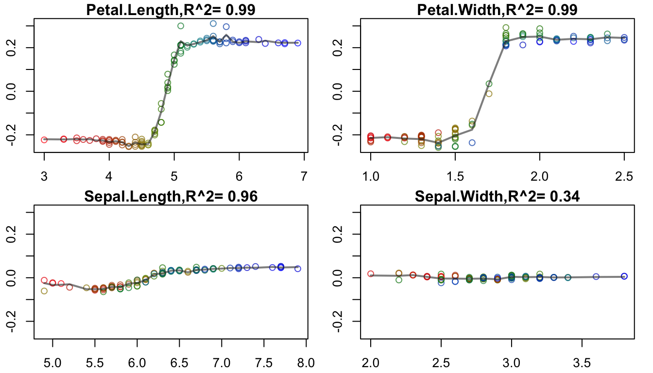
Top 6 RF feature contributions to the predictions, as exported by forestFloor.
Based on the above plot, one can further examine the interaction effect of the top 2 contributor features. This is accomplished via the forestFloor::show3d function:
# Interfacing with rgl::plot3d :
show3d(ff,1:2,col=Col,plot.rgl.args = list(size=2,type="s",alpha=.5))
rgl::rglwidget()3d interaction effect in the prediction contribution of the top 2 RF features.
# End of forestFloor::forestFloor documentation.
The interaction effect is clearly visible: As Petal.Length and Petal.Width both increase in value, their combined contribution to the Random Forest prediction also rises. Here, the combined contribution is defined as the sum of the marginal contributions i.e. the default value in forestFloor::show3d. The result is an insightful and useful depiction of the interaction effect.
However, this is a contrived example with just a handful of data points to depict. It is also shown here primarily for illustration purposes. A real use case scenario could quite possibly render such visualisations very hard to depict due to the issues previously mentioned.
At this point we can start exploring the combined contribution of any 2 way interactions with vis2rfi. As is explained in forestFloor, a low R-squared value for the goodness of fit of a particular feature (as with Sepal.Width in the facetted plot above) indicates the presence of a 2 way significant effect with another feature. Indeed, forestFloor aims at uncovering 2 way latent interactions, and this is one of its key strengths.
For the moment, we stick with the top 2 RF features and further explore their interaction.
We take a 25% subsample of the data, which is the default rsf argument value of the package’s main function vis2rfi::vis2rfi, and similarly examine the interaction effect of the first two most important variables. In addition we do not standardize the inputs but we do change the default combined contribution function from multiplication to addition.
# Loading and attaching the package:
library(vis2rfi)
#R> Loading required package: plotly
#R> Loading required package: ggplot2
#R>
#R> Attaching package: 'ggplot2'
#R> The following object is masked from 'package:randomForest':
#R>
#R> margin
#R>
#R> Attaching package: 'plotly'
#R> The following object is masked from 'package:ggplot2':
#R>
#R> last_plot
#R> The following object is masked from 'package:stats':
#R>
#R> filter
#R> The following object is masked from 'package:graphics':
#R>
#R> layout
#R>
#R> VV VV II SSSS 2222 RRRR FFF II
#R> VV VV II SSS 22 R R F II
#R> VV VV II SSS 22 RRR FFF II
#R> VVV II SSSS 2222 R R F II
#R>
#R> vis2rfi : Visualising 2Way Random Forest Interactions
#R> A main theme of this package is to repeatedly explore the interaction effect of two variables (i.e. 2 way) after running the Random Forests algorithm in supervised mode (currently binary classification is only tested). Experiment with the different subsampling approaches depending on the size of your data. As a reminder, make sure you have run function forestFloor from the forestFloor package on your data, as vis2rfi is currently using the feature contributions to the prediction from this package.
#R>
vis2rfi(impInd = c(1,2), ffObj = ff, rsf = 0.25, scaleXY = FALSE, outer = list(FUN = "+"))
#R> Taking the random subsample.
#R> An rsf value of 0.25 corresponds to 25 cases, out of the 100 ones.
#R> Computing the 3d visualization.3d interaction effect in the prediction contribution of the top 2 RF features, using a 25% subsample.
Remarks on the above output :
- Visualization is a structure-like object composed of various data slices. This is in contrast to a single surface view, as was previously mentioned in package premise.
- Easy to turn around and examine at any angle.
- Rich in colorfulness and interactivity, since leveraging the plotly package.
- Contour lines, as well as data point interactivity, help in discovering areas of both low and high contribution.
- The interaction effect is similarly found as before but with an important difference: There are also data points exhibiting a high contribution but with both Petal.Length and Petal.Width having mid-to-low values. Place for example the mouse cursor on the object’s apex and observe the red lined contours appearing on the feature plane.
Such cases are more evident when viewing the interaction effect in this manner since their contribution is not as attenuated as when plotting all of the data. The premise underlying vis2rfi is that 2 way interaction effects, when viewed as a 3d object as opposed to a single surface, can be easier discovered and further examined in a richer manner. Furthermore, taking data subsamples and visually experimenting with them is an idea well rooted in statistical thinking.
Let’s take a different subsample, by changing the seed.
vis2rfi(impInd = c(1,2), ffObj = ff, rsf = 0.25, scaleXY = FALSE, seed = 007, outer = list(FUN = "+"))
#R> Taking the random subsample.
#R> An rsf value of 0.25 corresponds to 25 cases, out of the 100 ones.
#R> Computing the 3d visualization.3d interaction effect in the prediction contribution of the top 2 RF features, using the default 25% subsample, without variable standardization and a different random seed.
A bit different shape is observed but with similar conclusions to the last plot above. This is due to the small size of this data set. In less contrived scenarios the difference can be more intense as the effect from a markedly different subspace is explored.
Taking a random subsample does not guarantee having a variety of contribution values in the subsample. To account for this we can use the maxDissim argument so as to include in the subsample data points that better span the variety of values observed in the initial data set. While this is shown below, note that maxDissim=TRUE argument implements a progress bar that’s not indicated on this vignette, but would appear when running the code on the R console. This is a visual feature leveraging the progress R package.
vis2rfi(impInd = c(1,2), ffObj = ff, rsf = 0.25, scaleXY = FALSE, maxDissim = TRUE, outer = list(FUN = "+"))
#R> Taking the random subsample.
#R> An rsf value of 0.25 corresponds to 25 cases, out of the 100 ones.
#R> Taking the random base 0.67 & pool 0.33 subsample percentage of rsf = 0.25 for maxDissim.
#R> Base subsample size is :
#R> 17 cases
#R> Pool subsample size is :
#R> 83 cases
#R> Computing the maxDissim object.
#R> Adding to base subsample 8 cases from the pool subsample, for a total of 25 cases.
#R> Computing the 3d visualization.3d interaction effect in the prediction contribution of the top 2 RF features, with defaults except with sampling more extreme cases in the data and without variable standardization.
Now the distinction in combined contribution between high and low values of the variables is also visible in other parts of the feature plane. Similarly as before, these can be viewed by placing the mouse cursor on the 3d object’s apex. Note also how the depicted object has altered it’s structure over these newly identified regions of interest at say point (x = 6.9, y = 1.4).
If we take another data view, by changing the seed value, we can see this distinction a bit better.
vis2rfi(impInd = c(1,2), ffObj = ff, rsf = 0.25, scaleXY = FALSE, maxDissim = TRUE, seed = 007, outer = list(FUN = "+"))
#R> Taking the random subsample.
#R> An rsf value of 0.25 corresponds to 25 cases, out of the 100 ones.
#R> Taking the random base 0.67 & pool 0.33 subsample percentage of rsf = 0.25 for maxDissim.
#R> Base subsample size is :
#R> 17 cases
#R> Pool subsample size is :
#R> 83 cases
#R> Computing the maxDissim object.
#R> Adding to base subsample 8 cases from the pool subsample, for a total of 25 cases.
#R> Computing the 3d visualization.3d interaction effect in the prediction contribution of the top 2 RF features, with defaults except sampling more extreme cases in the data, without variable standardization and using a different random seed.
Observe how at the same data point i.e. (x = 6.9, y = 1.4), the object’s “roof” tilts more vividly than in the previous visualisation.
The main theme of vis2rfi is to repeatedly alter the function’s parameters so as to view the 2 way contribution from a variety of perspectives, as shown for example here. The added benefit of doing this is expected to be more prominent in situations having a larger data size and/or a less easily established 2 way contribution to the predicted target.
Smoothing The Combined Feature Contribution 3D Object Into A Surface
Visualising 3d objects can be helpful in extracting detailed insights of an important 2 way contribution. Sometimes though we would like to isolate the interaction effect so as obtain a clearer picture, which can then be shown to a less technical audience.
We can portray the effect by a smoothed 3d surface that immediately shows us the important interaction and with a tilt towards the variable that contributes the most i.e. Petal.Length here, having a median marginal feature contribution of 0.85% as opposed to Petal.Width with a median of -15.34%.
GAM technology is utilized in order to conduct the smoothing, and the default smoothing parameters in argument df are 4 degrees of freedom for each of the features.
vis2rfi(impInd = c(1,2), ffObj = ff, rsf = 0.25, scaleXY = FALSE, maxDissim = TRUE, seed = 007, outer = list(FUN = "+"), smoother = TRUE)
#R> Taking the random subsample.
#R> An rsf value of 0.25 corresponds to 25 cases, out of the 100 ones.
#R> Taking the random base 0.67 & pool 0.33 subsample percentage of rsf = 0.25 for maxDissim.
#R> Base subsample size is :
#R> 17 cases
#R> Pool subsample size is :
#R> 83 cases
#R> Computing the maxDissim object.
#R> Adding to base subsample 8 cases from the pool subsample, for a total of 25 cases.
#R> Fitting the GAM smoothing spline with 4 and 4 degrees of freedom respectively on each of the two interaction variables.
#R> Computing the 3d visualization.3d interaction effect in the prediction contribution of the top 2 RF features, with defaults except smoothing with 4 degrees of freedom, sampling more extreme cases in the data, without variable standardization and using a different random seed.
More succinctly than without smoothing, the surface’s high upwards incline depicts the increase in the contribution to the prediction. In addition, the interaction effect has been established with only a 25% subset of the data. In many practical applications this is enough to convey the message.
If we would like to further emphasize the interaction effect, we can flatten the 3d surface by lowering the smoothing spline degrees of freedom in the GAM fit to unit values i.e.
vis2rfi(impInd = c(1,2), ffObj = ff, rsf = 0.25, scaleXY = FALSE, maxDissim = TRUE, seed = 007, outer = list(FUN = "+"), smoother = TRUE, df = c(1,1))
#R> Taking the random subsample.
#R> An rsf value of 0.25 corresponds to 25 cases, out of the 100 ones.
#R> Taking the random base 0.67 & pool 0.33 subsample percentage of rsf = 0.25 for maxDissim.
#R> Base subsample size is :
#R> 17 cases
#R> Pool subsample size is :
#R> 83 cases
#R> Computing the maxDissim object.
#R> Adding to base subsample 8 cases from the pool subsample, for a total of 25 cases.
#R> Fitting the GAM smoothing spline with 1 and 1 degrees of freedom respectively on each of the two interaction variables.
#R> Computing the 3d visualization.3d interaction effect in the prediction contribution of the top 2 RF features, with defaults except with linear smoothing, sampling more extreme cases in the data, without variable standardization and using a different random seed.
Resulting in a 3d plane for this data set while the tilt towards Petal.Length is more evident.
Example After Fitting With caret package
This is another example also coming from forestFloor documentation.
rm(list=ls())
library(caret)
#R> Loading required package: lattice
# Loading required package: lattice
#
# Attaching package: ‘caret’
#
# The following objects are masked from ‘package:vis2rfi’:
#
# minDiss, sumDiss
library(forestFloor)
N = 1000
vars = 7
noise_factor = .3
bankruptcy_baserate = 0.2
X = data.frame(replicate(vars,rnorm(N)))
y.signal = with(X,X1^2+X2^2+X3*X4+X5+X6^3+sin(X7*pi)*2) # some non-linear f
y.noise = rnorm(N) * sd(y.signal) * noise_factor
y.total = y.noise+y.signal
y = factor(y.total>=quantile(y.total,1-bankruptcy_baserate))
set.seed(1)
caret_train_obj <- train(
x = X, y = y,
method = "rf",
keep.inbag = TRUE, # always set keep.inbag=TRUE passed as ... parameter to randomForest
ntree=50, # speed up this example, if set too low, forestFloor will fail
)
rf = caret_train_obj$finalModel #extract model
if(!all(rf$y==y)) warning("seems like training set have been resampled, using smote?")
# simply pass train
ff = forestFloor(caret_train_obj,X,binary_reg = T)
#R> This seems to be an caret object. Trying to extract 'randomForest' model
#R> caret support is experimental, see help(forestFloor) for an example with caret
#R> ask/complain freely at https://github.com/sorhawell/forestFloor/issues/27
#R> [1] "RF is classification, converting factors/categories to numeric 0 an 1"
#R> defining FALSE as 0
#R> defining TRUE as 1[1] " "
#R> [1] "setting calc_np=TRUE"
plot(ff,1:6,plot_GOF = TRUE)
#R> [1] "compute goodness-of-fit with leave-one-out k-nearest neighbor(guassian weighting), kknn package"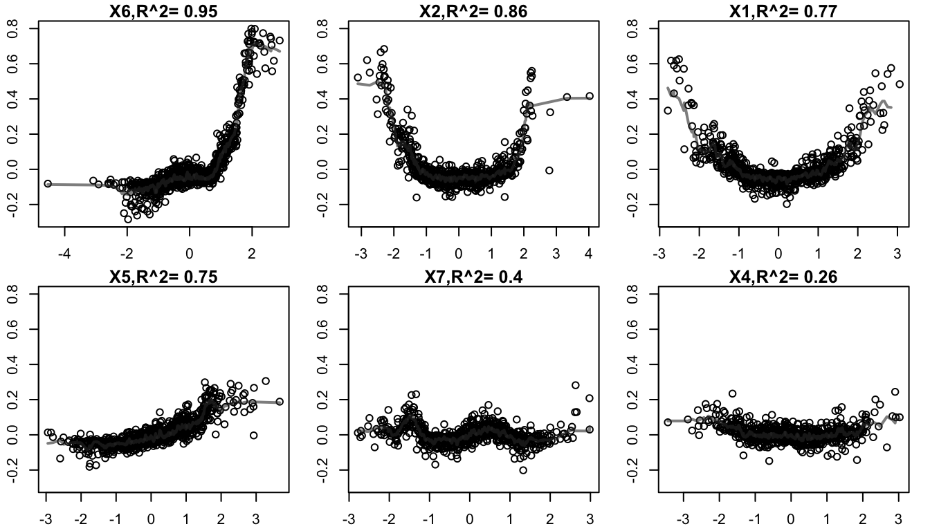
Main effects in prediction contribution of the top 6 RF features, as exported by forestFloor.
For example, we focus on the 6th in order of importance variable since it has the lowest R-squared goodness of fit value. Then we explore its interaction with the 7th most important variable in the Random Forest. These variables correspond to the x3 and x4 variables respectively, which are known to interact:
# library(vis2rfi) # If not already run.
vis2rfi(impInd = c(6,7), ffObj = ff, scaleXY = FALSE, outer = list(FUN = "+"))
#R> Taking the random subsample.
#R> An rsf value of 0.25 corresponds to 250 cases, out of the 1000 ones.
#R> Computing the 3d visualization.3d interaction effect in the prediction contribution between the the top 6th and 7th RF features. Marginal contributions are summed and without variable standardization.
Next we utilize a smoother :
vis2rfi(impInd = c(6,7), ffObj = ff, scaleXY = FALSE, maxDissim = TRUE, outer = list(FUN = "+"), smoother = TRUE)
#R> Taking the random subsample.
#R> An rsf value of 0.25 corresponds to 250 cases, out of the 1000 ones.
#R> Taking the random base 0.67 & pool 0.33 subsample percentage of rsf = 0.25 for maxDissim.
#R> Base subsample size is :
#R> 170 cases
#R> Pool subsample size is :
#R> 830 cases
#R> Computing the maxDissim object.
#R> Adding to base subsample 80 cases from the pool subsample, for a total of 250 cases.
#R> Fitting the GAM smoothing spline with 4 and 4 degrees of freedom respectively on each of the two interaction variables.
#R> Computing the 3d visualization.3d interaction effect in the prediction contribution between the the top 6th and 7th RF features. Smoothing and sampling more extreme cases in the data are also added to the run above.
And with multiplying the contributions i.e. the true functional relationship in the interaction :
vis2rfi(impInd = c(6,7), ffObj = ff, scaleXY = FALSE)
#R> Taking the random subsample.
#R> An rsf value of 0.25 corresponds to 250 cases, out of the 1000 ones.
#R> Computing the 3d visualization.3d interaction effect in the prediction contribution between the the top 6th and 7th RF features. Function run is with defaults except without variable standardization.
vis2rfi(impInd = c(6,7), ffObj = ff, scaleXY = FALSE, smoother = TRUE)
#R> Taking the random subsample.
#R> An rsf value of 0.25 corresponds to 250 cases, out of the 1000 ones.
#R> Fitting the GAM smoothing spline with 4 and 4 degrees of freedom respectively on each of the two interaction variables.
#R> Computing the 3d visualization.3d interaction effect in the prediction contribution between the the top 6th and 7th RF features. Function run is with defaults except without variable standardization and with smoothing.
vis2rfi(impInd = c(6,7), ffObj = ff, scaleXY = FALSE, maxDissim = TRUE, smoother = TRUE, df = c(1,1))
#R> Taking the random subsample.
#R> An rsf value of 0.25 corresponds to 250 cases, out of the 1000 ones.
#R> Taking the random base 0.67 & pool 0.33 subsample percentage of rsf = 0.25 for maxDissim.
#R> Base subsample size is :
#R> 170 cases
#R> Pool subsample size is :
#R> 830 cases
#R> Computing the maxDissim object.
#R> Adding to base subsample 80 cases from the pool subsample, for a total of 250 cases.
#R> Fitting the GAM smoothing spline with 1 and 1 degrees of freedom respectively on each of the two interaction variables.
#R> Computing the 3d visualization.Function run is with defaults except without variable standardization. Function run is with defaults except without variable standardization, with linear smoothing and sampling more extreme cases in the data.